Metapopulation

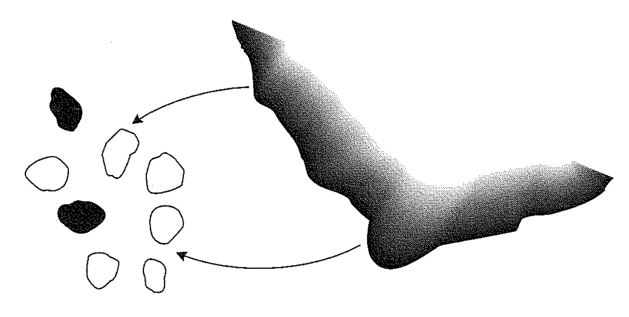
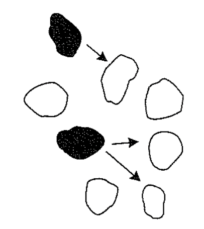
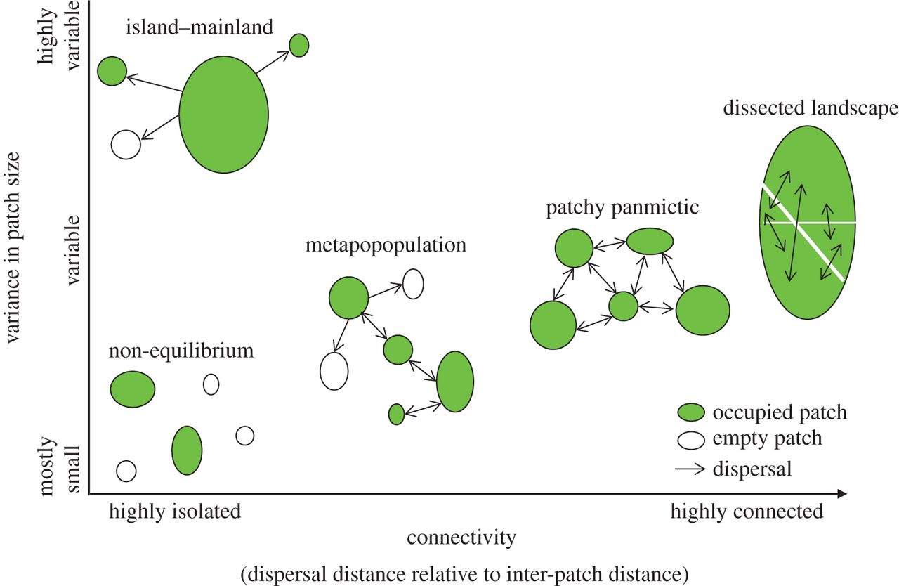
# Metapopulation
### Daijiang Li
### LSU

---

## Exam 1

---

# Population dynamics so far

.font200[
- Exponential growth with unlimited resource
- Logistic growth (Carry Capacity _K_)
- Age structures
- Closed population and dispersal
]

---

# Metapopulation

### The movement of individuals among sites can be potentially important to the persistence and survival of populations.

### *Metapopulation*: population of populations (Levins 1970); a group of several local populations linked by immigration and emigration

---

# Scaling populations to landscapes

.font200[
1. No longer focus on number of individuals (i.e. population size); instead we focus on the population's .red[_persistence_] (i.e., local extinction or local persistence)

2. Shift to focus on regional and landscape level with many connected sites; we no longer focus on the persistence of any particular population; instead we try to understand the .blue[_fraction of all population sites that are occupied_]
]

???

parking lot; does not care about a specific lot, but the proportion of opening/filled lots

---

# Local vs regional extinction risk

]

#### One population

`$p_e$`: probability of local extinction, e.g. `$p_e = 0.7$`

probability of persistence = `$1 - p_e$`, e.g., 0.3
]

#### Multiple (e.g., `$n = 5$`) population

probability of regional extinction = `$(p_e)^{n}$` = `$0.7^5$` = 0.16807

probability of regional persistence = `$1 - (p_e)^{n}$` = `$1 - 0.7^5$` = 0.83193
]

---

# Metapopulation models

## Assumptions

- no spatial structure

- no time lags: instantaneous response

- constant colonization/immigration and extinction rates

- regional occurrence affects local colonization and extinction rates

- large number of patches
]

---
class: center, middle

# Parameter symbols in notes vs book

|                            | Notes | Book |
|----------------------------|-------|------|
| Fraction of sites occupied | `$N$`     | `$f$`    |
| Colonization rate          | `$c$`     | `$p_i$`  |
| Extinction rate            | `$e$`    | `$p_e$`  |
]

`$p_i$`: is approximately the proportion of open sites colonized per unit time

`$p_e$`: the probability that a site becomes unoccupied per unit time
]

---

# Metapopulation models

`$$\frac{df}{dt}=I-E$$`

`$$I=p_i(1-f)$$`

`$$E = p_ef$$`

`$$\frac{df}{dt}= p_i(1-f)-p_ef$$`

### The above equation will serve as a template for developing alternative metapopulation models.

---

# The island-mainland model

.font150[
The equation in the previous slide is the simplest model for our metapopulation with `$p_i$` and `$p_e$` as constants.
- `$p_e$` is a constant so that the probability of extinction is the same for each population and does not depend on the fraction of patches occupied
- `$p_i$` is constant implies a **propagule rain**, a continuous .blue[external] source of migrants
]

---

# The island-mainland model

`$$\frac{df}{dt}=0=p_i(1-f)-p_ef$$`

`$$p_if+p_ef=p_i$$`

`$$\hat{f}=\frac{p_i}{p_i+p_e}$$`
]
]

### Note that even with large `$p_e$` and small `$p_i$` (it will always be >0 because of external sources), `$f$` will still > 0, i.e. at least some of the sites in the metapopulation will be occupied.

---

# Internal colonization (Levins model)

.font150[
No propagule rain and the only source of propagules for the metapopulation is the set of occupied sites, i.e., .red[internal colonization]
]

`$$p_i=if$$`

`$$\frac{df}{dt}=if(1-f)-p_ef$$`

]
]

---

# Internal colonization

## Find Equilibrium

1. set the equation `$\frac{df}{dt}=if(1-f)-p_ef$` to 0

2. solve `$f$`
]
]

`$$p_e=i-if$$`

`$$\hat{f}=\frac{i-p_e}{i}=1-\frac{p_e}{i}$$`

]
]

---

# The Rescue Effect

`$p_e$` might be affected by `$f$` because with higher `$f$` there would be more propagules that leave the site and may arrive at occupied sites to increase the local population size.

This increase in local population size `$N$` is a .red[rescue effect] that may prevent the local population from extinct due to demographic and environmental stochastics.
]

`$$\hat{f}=\frac{p_i}{e}$$`
]
]

---

# Neutral Equilibrium

### Internal colonization + Rescue effect

`$$\frac{df}{dt}=if(1-f)-ef(1-f)$$`

### Equilibrium?? No simple solution!

- `$i < e$`, metapopulation contracts until `$f=0$` (regional extinction)

- `$i = e$`, no change for `$f$`
]

---

# Types of metapopulation

![](figs/MP1.jpg)

---
class: center, middle

# Four metapopulation models

|                                        | Independent `$p_e$`             | `$p_e$` mediated by rescue effect  |
|----------------------------------------|-------------------------------|----------------------------------|
| External colonization (propagule rain) | `$\frac{df}{dt}=p_i(1-f)-p_ef$` | `$\frac{df}{dt}=p_i(1-f)-ef(1-f)$` |
| Internal colonization                  | `$\frac{df}{dt}=if(1-f)-p_ef$`  | `$\frac{df}{dt}=if(1-f)-ef(1-f)$`  |

<br>

|                                        | Independent `$p_e$`     | `$p_e$` mediated by rescue effect |
|----------------------------------------|-----------------------|---------------------------------|
| External colonization (propagule rain) | Island-mainland model | Rescue effect                   |
| Internal colonization                  | Levins model          | Neutral equilibrium             |